CS231n Backpropagation for convolutional neural network

This post briefly covers backpropagation for a convolutional neural network, derived in the context of work on the second assignment for the Winter 2016 iteration of the Stanford class CS231n: Convolutional Neural Networks for Visual Recognition.

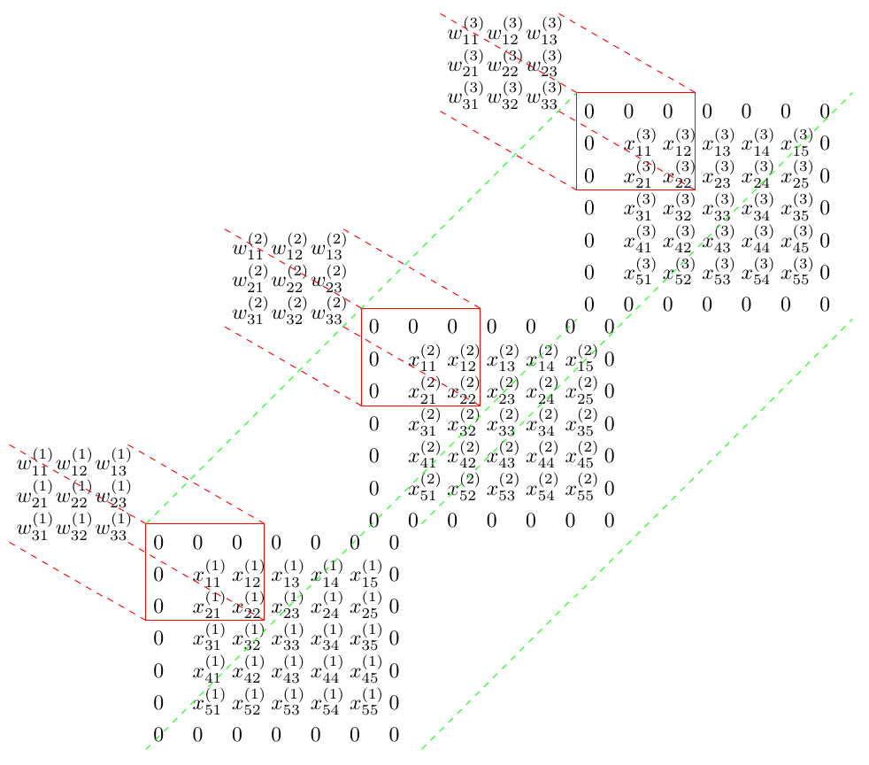
As in the assignment, the setting for this post is a convolutional layer with input size $X = \left( 4, 3, 5, 5\right)$, where the dimensions of the input refer to number of input observations $N$, input depth $C$, input height $H$ and input width $W$. The convolutional layer has two channels $F$, again a filter depth $C$ of three and also a filter height $HH$ and filter width $WW$ of three, corresponding to the weight tensor $W = \left(2, 3, 3, 3\right)$. The upstream derivative $dY = \left(4, 2, 5, 5\right)$ corresponds to the number of input observations $N$, number of channels $F$, and output height and width $H_{out}$ and $W_{out}$.

Let’s first make sense of the upstream derivative. For the convolutional layer, there are $F = 2$ different 3D filters, each of which convolves over the input (with zero-padding $P$ of size 1), using a stride $S$ of 1. The first step is to calculate the number of unique positions (and hence output volume) implied by the input size, filter size, stride and padding. This is easily calculated according to

$\begin{align} H_{out} &= (H−HH+2P)/S+1 & W_{out} &= (W−WW+2P)/S+1\\ &= (5 - 3 + 2 \times 1)/1 +1 & &= (5 - 3 + 2 \times 1)/1 +1\\ &= 5 & &= 5.\\ \end{align}$

Therefore, convolving over the input volume with the parameters described above involves taking a 3D dot product of the weights with the input volume at each of the $5 \times 5$ positions of the filter with respect to the input. This process is repeated with each of the $F = 2$ different filters, leading to an output volume of size $\left(2, 5, 5\right)$, and for each of the $N = 4$ observations, giving an output tensor $Y = \left(4, 2, 5, 5\right)$. Wonderful! This corresponds, as it should, to the dimensions of our upstream derivative $dY$, which is in fact the derivative of the loss with respect to the output volume of the convolutional layer, $\frac{d\mathcal{L}}{dY}$.

The key aim of the backpropagation derivation is to get from the derivative of the loss with respect to the output of the convolutional layer $Y$ to the quantities:

$dx$, the derivative of the loss with respect to the input to the convolutional layer
$dw$, the derivative of the loss with respect to the weights in the convolutional layer
$db$, the derivatives of the loss with respect to the biases in the convolutional layer

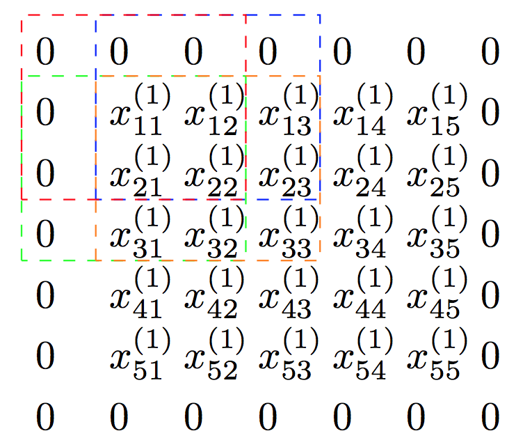
Remember how the convolution operation works. For the first observation and first filter, the first entry $y_{11}^{(1)}$ in the activation map is obtained by taking the 3D dot product of the weights with the first window in the zero padded input tensor. In basic Python, this corresponds to

output[0, 0, 0, 0] = np.sum(X[0, :, :3, :3] * W[0, :, :, :]) + b[0]

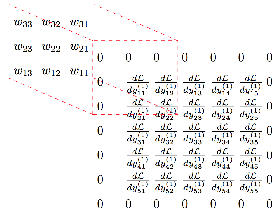
The operation can be visualised as the sum of 2D dot products across each of the three input dimensions according to the following diagram. To get to grips with the derivative of the loss with respect to the input of the convolutional layer $dx$, it was most helpful for me to first consider what was happening in the first input dimension, as this pattern repeats symmetrically in the other dimensions of the input depth. Let’s start small, and consider the derivative of the loss with respect to the first input in the first depth dimension, $x_{11}^{(1)}$. It’s relatively easy to see that given the filter size, stride and padding, there are four terms in the activation map for the first filter that include $x_{11}^{(1)}$: $y_{11}^{(1)}$, $y_{12}^{(1)}$, $y_{21}^{(1)}$ and $y_{22}^{(1)}$. These terms correspond to the application of the first filter at the spatial positions indicated below.

$y_{21}^{(1)}$, for instance, corresponds to the application of the first filter at the spatial position defined by the dashed green square. $y_{21}^{(1)}$ is the dot product

$\begin{align} y_{21}^{(1)} &= \sum_{d=1}^{3}\sum_{i=1}^{3}\sum_{j=1}^{3}xpad_{(1+i)j}^{(d)}w_{ij}^{(d)},\\ \end{align}$

where $xpad_{(1+i)j}^{(d)}$ is the $(1+i)j$th element of the zero-padded input array in the $d$th depth dimension. The only term in the expression for $y_{21}^{(1)}$ that contains $x_{11}^{(1)}$ is obtained at the index $(d=1, i=1, j=2)$, and so the derivative of this term with respect to the input, $\frac{dy_{21}^{(1)}}{dx_{11}^{(1)}}$, is $w_{12}^{(1)}$. Similarly breaking down the other terms in the activation map that include $x_{11}^{(1)}$ produces $\frac{dy_{11}^{(1)}}{dx_{11}^{(1)}}=w_{22}^{(1)}$, $\frac{dy_{12}^{(1)}}{dx_{11}^{(1)}}=w_{21}^{(1)}$ and $\frac{dy_{22}^{(1)}}{dx_{11}^{(1)}}=w_{11}^{(1)}$.

We can then use the chain rule to derive an expression for the derivative of the loss with respect to $x_{11}^{(1)}$ in terms of the convolutional weights and entries in the matrix of the upstream derivatives $\frac{d\mathcal{L}}{dY}$

$\begin{align} \frac{d\mathcal{L}}{dx_{11}^{(1)}} &= \sum_{i,\;j} \frac{d\mathcal{L}}{dy_{ij}^{(1)}} \times \frac{dy_{ij}^{(1)}}{dx_{11}^{(1)}}\\ &= \frac{d\mathcal{L}}{dy_{11}^{(1)}}\times w_{22}^{(1)} + \frac{d\mathcal{L}}{dy_{12}^{(1)}}\times w_{21}^{(1)} + \frac{d\mathcal{L}}{dy_{21}^{(1)}}\times w_{12}^{(1)} + \frac{d\mathcal{L}}{dy_{22}^{(1)}}\times w_{11}^{(1)}. \end{align}$

The key is then to recognise that the above sum corresponds to the application at the first spatial position of the first filter (with inverted weights) to the array of derivatives of the loss with respect to the output of the first filter, with zero padding of one. The diagram below shows this, and you can check for yourself that the derivatives of the loss with respect to the other inputs correpond to the application of the inverted filter to the zero-padded matrix at different spatial positions.

Naive implementation in Python is given below. Don’t forget we need to reproduce the convolution over all filters, observations and spatial positions.

dout_padded = np.pad(dout, ((0,0), (0,0), (conv_param['pad'],conv_param['pad']), (conv_param['pad'],conv_param['pad'])), 'constant')
  for i in range(N):
    for j in range(C):
      for k in range(H):
        for l in range(W):
          for m in range(F):
            dx[i, j, k, l] += np.sum(w[m, j, ::-1, ::-1] * dout_padded[i, m, (conv_param['stride'] * k): (conv_param['stride'] * k + HH), (conv_param['stride'] * l): (conv_param['stride'] * l + WW)])

Written on April 8, 2017